3. Coordinate Systems

Polar Coordinates

The polar coordinate system uses distances and directions to specify the location of a point in the plane and is set up with a fixed point , the pole, and a ray from called the polar axis. Each point can be assigned polar coordinates where is the distance of and is the angle between the polar axis and . Any point can also be represented by

for any integer .

The connection between the two systems of polar and rectangular coordinates is clear where polar axis coincides with the positive axis. Using trigonometric ratios, we can change from polar to rectangular coordinates:

To change from rectangular to polar coordinates, use

These equations do not uniquely determine or . Make sure the values chosen for and give a point in the correct quadrant.

Similar to how a rectangular equation is an equation in and , a polar equation is an equation in and . The graph of a polar equation uses a grid consisting of circles centered at the pole and rays emanating from the pole.

In general, the graph of is a circle of radius centered at the origin because it consists of all points whose coordinate is , and we see that the equivalent equation in rectangular coordinates is after squaring both sides of the equation.

To sketch a graph of the polar equation , we first determine the polar coordinates of several points on the curve

The same points would be obtained if we allowed to range from to since is negative in that range. We plot these points, then join them to sketch the curve and the graph appears to be a circle. To express in rectangular coordinates:

In general, the graph of an equation of the form

is a circle with radius centered at the points with polar coordinates and , respectively.

Graphing Polar Equations

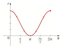
To graph some of the polar equations, instead of plotting points, we can first sketch the graph in rectangular coordinates for reference that enables reading at a glance the values of that correspond to a given . For example, the process of graphing is illustrated below.

Note the domain for in this case would be exactly : letting increase beyond or decrease beyond and we would be retracing the path. The heart-shaped curved is called a cardioid. In general, the graph of any equation of the form

is a cardioid.

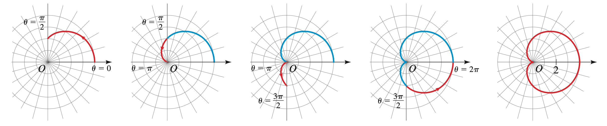
The curve can be graphed in a similar manner:

This curve has four petals and is called a four-leaved rose. In general, the graph of an equation of the form

is an leaved rose if is odd or a leaved rose if is even.

Symmetry

The graph of a polar equation is symmetric:

• with respect to the polar axis, if . Common triggers are equations involving only since .
• with respect to the pole, if , or . Graph should be unchanged when rotated radians about the pole. Common triggers are certain equations like the one above or equations where is squared, for example, .
• with respect to the line , if . Common triggers are equations involving only since .

In rectangular coordinates the zeros of the function correspond to the intercepts of the graph. In polar coordinates, the zeros of the function are the angles at which the curve crosses the pole. This is demonstrated in the following example of graphing :

This curve is called a limaçon (pronounced lih-muh-son, Middle French for snail). In general, the graph of an equation of the form

is a limaçon.

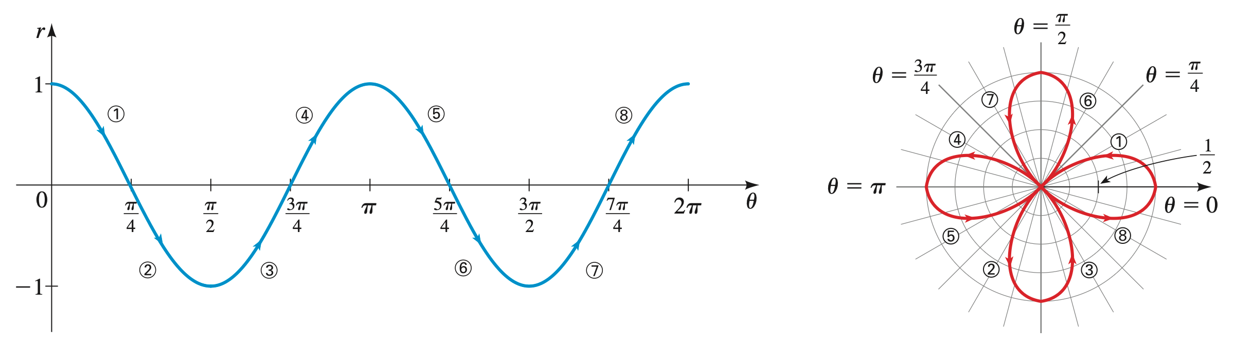
Consider the equation . We need to first determine the domain for , that is, finding the smallest interval that traces the entire curve without overlapping. The graph only repeats itself when the same value of is obtained at both and , thus we need to find the smallest integer that satisfies

For this equality to hold, must be a multiple of , therefore . In conclusion, we obtain the entire graph if we choose values between and .

Complex Numbers

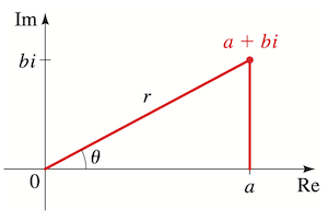
We graph real numbers using the number line, which has one dimension. The fact that complex numbers have two components: a real part and an imaginary part, suggests we need two axes to graph complex numbers: the real axis and the imaginary axis. The plane determined by these two axes is called the complex plane. The complex number is represented by ordered pair in this plane. Similar to how the absolute value of a real number can be thought of as its distance from the origin, we define that the absolute value (or modulus) for complex number is

which is also the length of the line segment joining the origin to the point in the complex plane. If is an angle in standard position whose terminal side coincides with the line segment, we have

where and . is called the argument of . This is the polar form of the complex number in which the multiplication and division operations can be simplified:

which leads us to the De Moivre’s Theorem:

An th root of a complex number is a complex number such that . De Moivre’s Theorem suggests one th root of would be

The argument of can be replaced by for any integer , which would make the expression give a different value of for . Therefore, for any positive integer , complex number has distinct th roots

where the modulus of each th root is , the argument of the first root is . Repeatedly add to get the argument of each successive root. These observations show that the th roots of are spaced equally on the circle of radius when graphed.

Parametric Equations

Parametric Equations are a general method for describing any curve. Think of a curve as the path of a point moving in the plane; the and coordinates of the point are functions of time:

These equations are parametric equations for the plane curve that is the set of points , where , with parameter . A curve given by parametric equations can also be represented by a single rectangular equation with a process called eliminating the parameter. For example, consider the parametric equations

Solving for and substituting into the equation for , we get

Thus the curve is a parabola. Eliminating the parameter often helps us identify the shape of a curve. For another example:

Notice that , and since all points on the curve given by the parametric equations satisfy this equation, so the graph is a circle of radius centered at the origin. As increases from to , the point starts at and moves counterclockwise once around the circle.

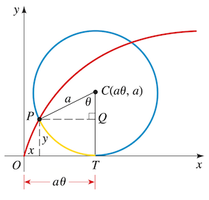
We cover another example. As a circle of radius rolls along the axis, the curve traced out by a fixed point on the circumference is a cycloid for which we try to find the parametric equations. Let be the angle the circle has rolled through with the point started from the origin.

The distance that the circle has rolled must be the same as the length of the arc . From the figure we see

Vectors

A quantity determined completely by their magnitude, for example, mass, temperature and energy, is called a scalar. Quantities such as displacement, velocity and force that involve magnitude as well as direction are called directed quantities, which we represent through vectors. A vector in the plane is a line segment with an assigned direction, its length is called the magnitude. A vector denoted by (we often use boldface letter to denote vectors, so ) has initial point and terminal point .

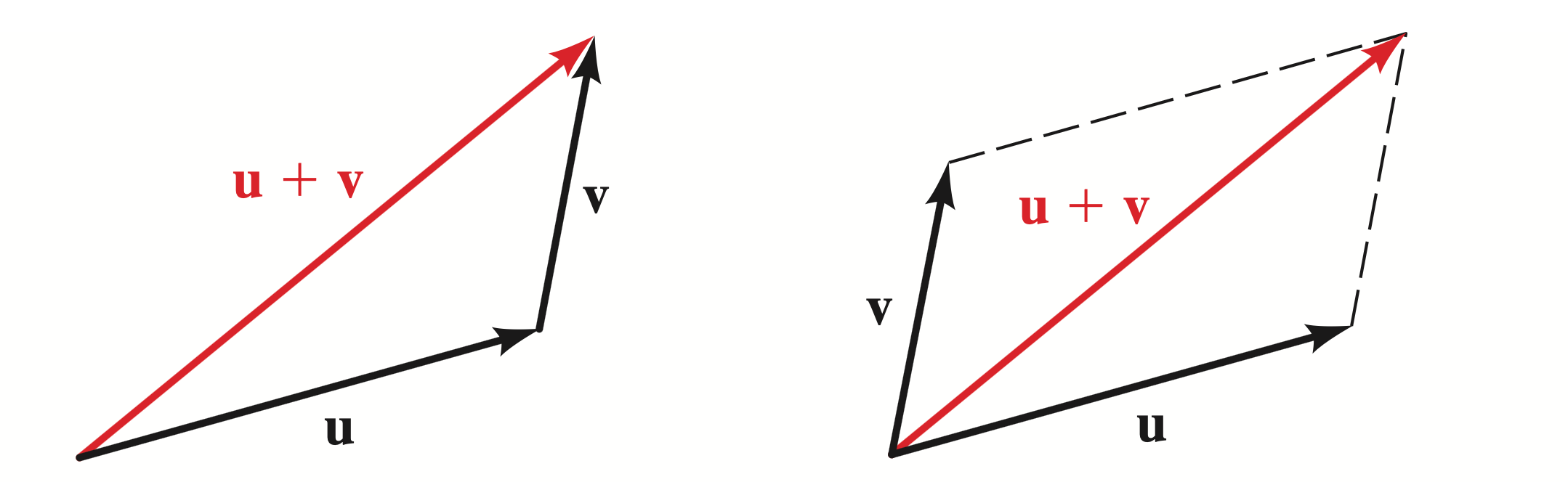
To find the sum of any two vectors and , we sketch vectors equal to and with the initial point of one at the terminal point of the other, or if drawn starting at the same point, and would be the vector that is the diagonal of the parallelogram formed.

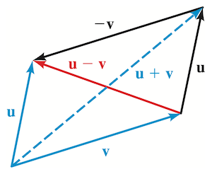
Multiplying a vector by a scalar has the effect of stretching or shrinking the vector. We define that the vector where is a real number has magnitude and has the same direction as if . The difference of two vectors and is defined by , as illustrated.

We can also describe vectors analytically by placing them in a coordinate plane, and represent them as ordered pairs of real numbers. Suppose we move units to the right and units upward to go from the initial point of the vector to the terminal point, then

where is the horizontal component of and is the vertical component of . It follows that if a vector is represented in the plane with initial point and terminal point , then

Note the vector is not the point . The vector itself represents only a magnitude and a direction, not a particular arrow in the plane, and therefore has many different representations depending on its initial point.

Two vectors are considered equal if they have equal magnitude and the same direction. In other words, two vectors are equal if and only if their corresponding components are equal, that is, for the vectors and , and .

The magnitude of a vector is

A unit vector is a vector of length . For instance, is a unit vector. Two special unit vectors are and defined by

We can express vectors in terms of them:

If we let be in the plane with its initial point at the origin, with a direction of , then

Thus we can also express as

We define the dot product of two vectors and to be

To get a dot product, the corresponding components are multiplied then added, resulting in a scalar instead of a new vector. Also notice the property

Let and be in the plane with their initial points at the origin, be the smaller of the angles formed by the two vectors, thus . Applying the Law of Cosines to the triangle formed by , and , and using the above property we get

Thus

where is the angle between the two nonzero vectors and . This is the Dot Product Theorem. Solving for , we get

which allows us to find the angle between two vectors by their components.

Two nonzero vectors and are called perpendicular if the angle between then is , and in that case,

Thus two nonzero vectors are perpendicular if and only if their dot product equals to .

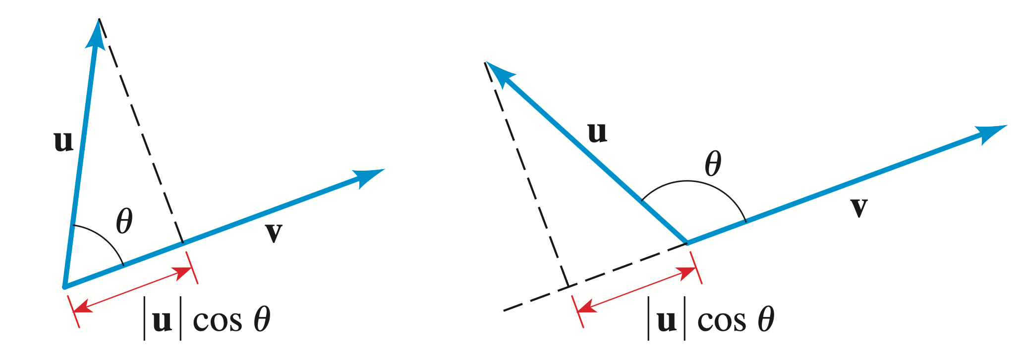
We define the component of along (or the scalar projection of onto ) to be

where is the angle between and . Intuitively, the component of along is the magnitude of the portion of that points in the direction of . The below figure illustrates this concept.

In short, the component of along is

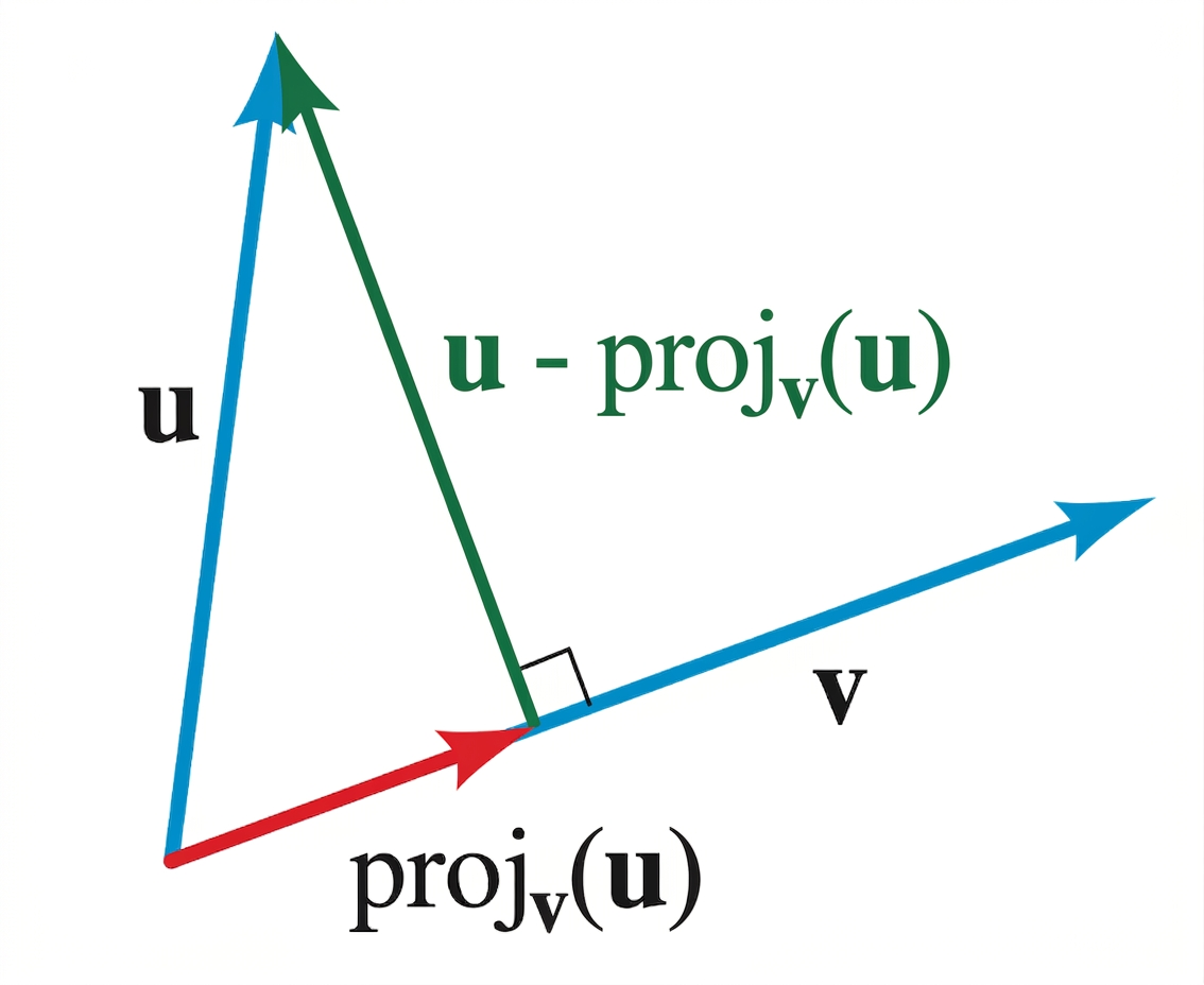
The vector parallel to and whose length is the component of along is the projection of onto , given by

We often need to resolve a vector into the sum of two vectors, one parallel to and one orthogonal to in the form of , and in this case,

The below figure illustrates the idea.

For example, let and , then . If we resolve into and where is parallel to and is orthogonal to , then and .

Systems of Equations

Systems of Linear Equations

A linear equation in variables can be put in the form

where and are real numbers and are variables.

A system of equations is a set of equations involving the same variables. A solution of a system is an assignment of values for the variables that makes each equation in the system true. To solve a system means to find all solutions and for a system of linear equations, we often use the elimination method to change it to an equivalent system, that is, a system with the same solutions as the original system, using the following operations that yield an equivalent system:

1. Add a nonzero multiple of one equation to another
2. Multiply an equation by a nonzero constant
3. Interchange the positions of two equations

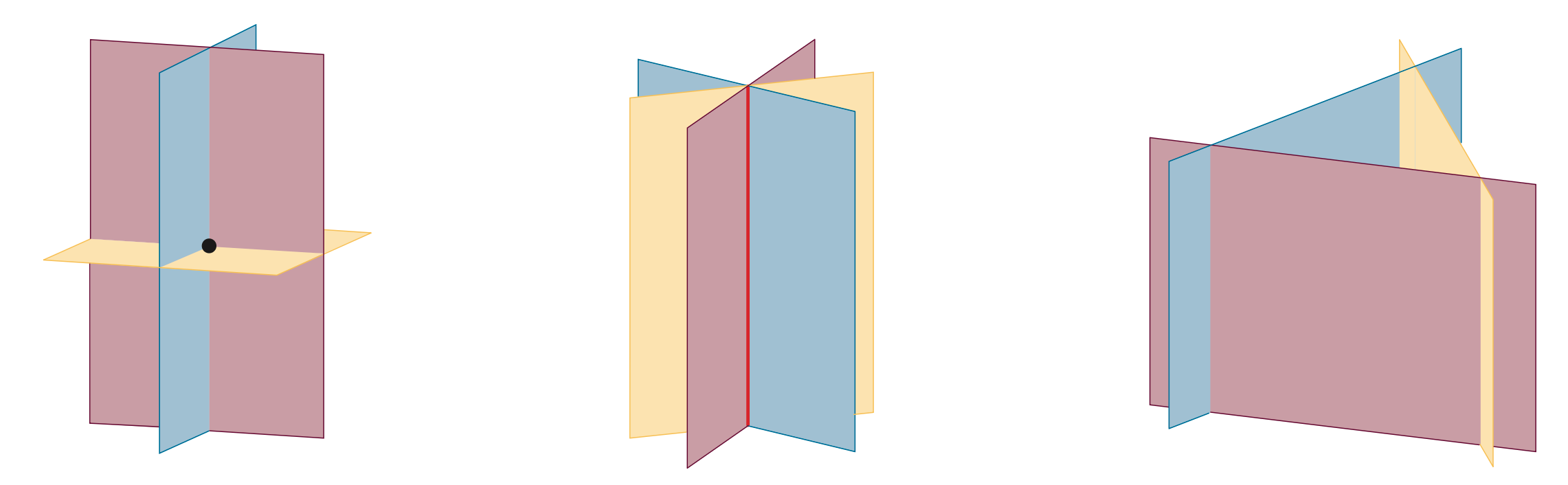
The graph of a linear equation in three variables is a plane in three-dimensional space, so a system of three such equations represents three planes in space, and the solutions are the points where all three planes intersect. The three planes may intersect at a single point, intersect along a line or have no point in common at all. As a result, a system can have exactly one solution, no solution or infinitely many solutions.

A system with no solution is said to be inconsistent and results in a false equation in the form of after applying Gaussian elimination to the system. A system with infinitely many solutions is said to be dependent.

A matrix is a rectangular array of numbers used to organize information into categories corresponding to the rows and columns of the matrix. We define an matrix is a rectangular array of numbers with rows and columns with dimension :

The numbers are the entries of the matrix where the subscript indicates that the entry is in the th row and th column. The matrices and are equal if and only if they have the same dimension and corresponding entries are equal, that is, . Similarly, two matrices can only be added or subtracted if they have the same dimension, we add or subtract the matrices by adding or subtracting corresponding entries:

The scalar product is the same matrix obtained by multiplying each entry of by :

The product (or ) of two matrices and is defined only when the number of columns in is equal to the number of rows in . Suppose the two matrices have these dimensions:

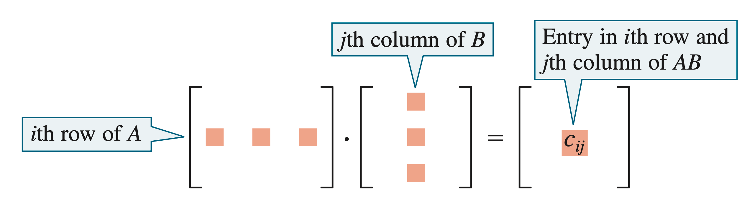
we see the two inner numbers must match for to be defined. The result of the product is a matrix of dimension (taken from the two outer numbers), as such, the resulting matrix has the same number of rows as and the same number of columns as . In fact, to obtain , we need to think of the row of and the column of as vectors. The dot product of the two vectors is an entry of the matrix . We define that if is an matrix and is an matrix, then their product is the matrix

where the entry in the th row and th column is the number obtained by multiplying corresponding entries of the th row of and the th column of and adding the results.

Matrix multiplication is not commutative, and is not necessarily defined since the inner numbers may not match, but even if is defined, it is not necessarily equal to .

Recall that the multiplicative identity is . Similarly, we define the identity matrix to be the square matrix for which each main diagonal entry (the entries whose row and column numbers are the same) is a and for which all other entries are , which behaves like the multiplicative identity in the sense that

If the product of two matrices of the same dimension is equal to , then we say that one is the inverse of the other. This concept of the inverse of a matrix is analogous to that of the reciprocal of a real number. If there exists a matrix with the property that

then is invertible and is the inverse of . We use the following rule to find the inverse of a matrix:

where the quantity is called the determinant of the matrix. If the determinant is , the matrix does not have an inverse.

A linear system is presented by what is called the augmented matrix. For example, the following linear system

may be represented by the augmented matrix

which contains the same information as the system. We use the same operations used in the elimination method for row operations on the augmented matrix of a system. These are called the elementary row operations and are described by these notations:

1. : Add times the th row to the th row.
2. : Multiply the th row by .
3. : Interchange the th and th rows.

We use a process called Gaussian elimination (in honor of its inventor, C. F. Gauss) to change a linear system to an equivalent triangular system then use back-substitution to solve the system, beginning with using the elementary row operations to put the matrix in row-echelon form: the leading entry (first nonzero number) in each row should be and to the right of the leading entry in the row immediately above it. Rows consisting entirely of zeros should be at the bottom of the matrix. To do this, we obtain a leading then obtain zeros below that on the first row, then move onto the next rows.

A matrix is in reduced row-echelon form if it is in row-echelon form, and every number above and below each leading entry is . Using the reduced row-echelon form to solve a system is called Gauss-Jordan elimination, which shows the solutions without the need for back-substitution. To put a matrix in reduced row-echelon form, we obtain zeros above each leading entry by adding multiples of the row containing that entry to the rows above it. We begin with the last leading entry and work upward. For example, to solve

we first write the augmented matrix of the system:

Using the elementary row operations we should arrive at

We then continue using elementary row operations to get

which shows the solution is .

A leading variable in a linear system is one that corresponds to a leading entry in the row-echelon form of the augmented matrix of the system. A inconsistent system with no solution in row-echelon form contains a row that represents the equation . On the other hand, a dependent system with infinitely many solutions has variables in the row-echelon form that are not all leading variables, and is not inconsistent, in which case we would have to express the leading variables in terms of the nonleading variables which may take on any real numbers as their values. For example, such a system may look like

The third row corresponds to the equation , which is always true and adds no new information. We solve for the leading variables and in terms of the nonleading variable :

To obtain the complete solution, we let be any real number and express , and in terms of :

Or, as the ordered triple where is any real number. This example illustrates a general fact: if a system in row-echelon form has nonzero equations in variables (), the complete solution will have nonleading variables. In this example we arrived at nonleading variable.

These techniques are also used for finding inverses for matrices in general. If is an matrix, we construct the matrix

that has the entries of on the left and of the identity matrix on the right which we then use the elementary row operations on to change the left side into the identity matrix (this means we are changing the large matrix to reduced row-echelon form), so it becomes

because the elementary row operations are essentially the same as multiplying by special matrices called elementary matrices:

where each is an elementary matrix corresponding to an elementary row operation. Since applying these operations turned into , that is, ,

so after the elementary row operations, the matrix becomes

Intuitively, we have arrived at the inverse of the matrix by recording the operations needed. However, if we encounter a row of zeros on the left side in the process, the original matrix does not have an inverse and is called singular.

A system of linear equations can also be written as a matrix equation in the form of

if the coefficient matrix has an inverse and if is a variable matrix and is a known matrix both with rows. We then use matrix operations to solve for the matrix to get . For example, the system

is equivalent to the matrix equation

We begin with the matrix whose left half is and whose right half is the identity matrix :

We then row-reduce the matrix so that the left half is transformed into the identity matrix:

which shows

Thus solution of the system is given by

That is, , and .

When we need to solve several systems of equations that have the same coefficient matrix, converting the systems to matrix equations provides an efficient way to obtain the solutions.

A square matrix can be assigned a number called its determinant which can be used to solve systems of linear equations, denoted by the symbol or . has an inverse if and only if .

If is a matrix, then ; and we have seen the determinant of a matrix is

To define the determinant for any arbitrary matrix , we say the minor of the element is the determinant of the matrix that is obtained by deleting the th row and the th column of , and the cofactor of the element is which is simply the minor of multiplied by or depending on whether is even or odd. In a matrix we may obtain the cofactor of any element by prefixing its minor with the sign obtained form the following checkerboard pattern:

For example, if is the matrix

then the minor

So the cofactor

In general, we define that the determinant of any square matrix is obtained by choosing any one row or any one column in , then multiplying each element of that row or column by its cofactor and adding the results:

For example, to show that

has no inverse, we calculate the determinant of . Notice all but one of the elements of the second row is zero, we expand the determinant by the second row. So

And since the determinant of is zero, cannot have an inverse. This example also shows the work can be reduced considerably if we expand a determinant about a row or column that contains many zeros. As such, we can often use the following principle to simplify the process of finding a determinant by introducing zeros into the matrix:

Determinants can sometimes be used to express the solutions of linear equations. Consider the following pair of linear equations:

Solving for and , and assuming , we get

which can be expressed using determinants as follows:

Let , notice the numerator of the fractions for and are simply determinants of with the first column or the second column replaced by and . So we use and to rewrite the solution of the system as

This can be extended to apply to any system of linear equations in variables in which the determinant of the coefficient matrix is not zero. We write the system as

where is the coefficient matrix. We let be the matrix obtained by replacing the th column of by the matrix , the solution of the system is then given by

Using determinants to solve systems of linear equations can be a useful alternative to Gaussian elimination but only in some situations. For example, in systems with more than three equations, evaluating the various determinants is usually inefficient.

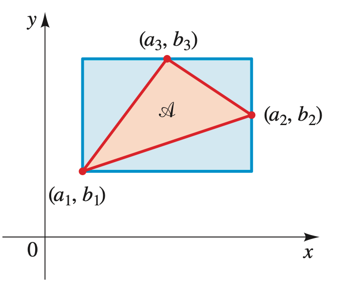
Determinants also provide a simple way to calculate the area of a triangle in the coordinate plane. If the triangle has vertices , and , as shown in the figure below,

it can be shown using algebra that the area of the triangle is